Flood Fill Mazes

Ian Ward · July 7, 2023

Python

In this article we generate mazes using jupyter notebooks, numpy, matplotlib, and the scikit-image flood_fill function.

Almost since I could first draw I’ve been fascinated with creating and solving mazes. Graph paper and mechanical pencils were some of my favorite gifts. Recently I’ve rediscovered some of that same childlike excitement by designing a homebrew cpu, and the next game I’m building for it needs some custom mazes.

There are lots of existing maze generating algorithms but I wanted something that filled cells (not grid edges) and that is fast and simple to do in Python so it would be easy to tweak and customize.

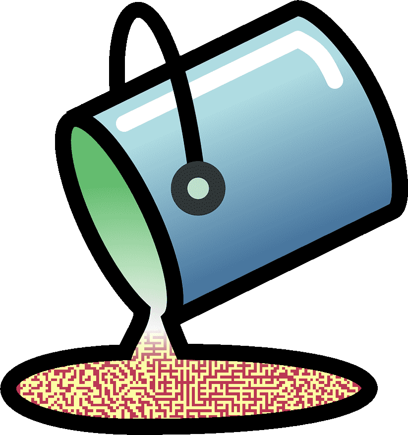
“Flood fill” functions work like the paint bucket tool in an image editing program. They start from one pixel in an image then expand to all connected pixels of the same color, replacing them with a new color.

If we start a flood fill from any pixel in an image and it covers all pixels with the same color then they must all be connected, like the path in a maze from the beginning to the end.

Dependencies

First install jupyter and a few common Python libraries, and launch jupyter notebook:

$ pip install jupyter matplotlib scikit-image
$ jupyter-notebook

This jupyter notebook file includes all examples in the article:

• Flood fill maze generation jupyter notebook file

We use numpy for efficient array operations, matplotlib for visualization, and scikit-image for image manipulation. Imports are at the top of the project, as usual. If you get any errors running these imports make sure you have the dependencies above installed:

import numpy as np
import matplotlib.pyplot as plt
import matplotlib.patches as mpatches
import matplotlib as mpl
from skimage.segmentation import flood_fill
from skimage.io import imread, imsave
from skimage.color import rgb2gray
from skimage.transform import resize
from skimage.filters import threshold_local

Square one

Our maze needs a border wall, a starting location, and an ending location. Let’s represent our maze with a numpy array where the border wall is marked with 1’s, the starting and ending locations are marked with 2’s and everything else is set to 0.

We follow numpy’s (y, x) convention for coordinates, so our “box” height comes first:

def box(height, width):
    arr = np.zeros((height, width), dtype=np.uint8)
    # walls top, bottom, left, right = 1
    arr[0] = arr[-1] = arr[..., 0] = arr[..., -1] = 1
    # start and end locations = 2
    arr[0, 1] = arr[-1, -2] = 2
    return arr

b = box(6, 6)
b

array([[1, 2, 1, 1, 1, 1],
       [1, 0, 0, 0, 0, 1],
       [1, 0, 0, 0, 0, 1],
       [1, 0, 0, 0, 0, 1],
       [1, 0, 0, 0, 0, 1],
       [1, 1, 1, 1, 2, 1]], dtype=uint8)

Let’s visualize our array with matplotlib. Choosing “inferno” as a nice a bright palette, we create a legend with color patches, and draw arrays with this “show” function:

palette = mpl.cm.inferno.resampled(3).colors
labels = ["0: unfilled", "1: wall", "2: passage"]

def show(arr):
    plt.figure(figsize=(9, 9))
    im = plt.imshow(palette[arr])
    # create a legend on the side
    patches = [mpatches.Patch(color=c, label=l) for c, l in zip(palette, labels)]
    plt.legend(handles=patches, bbox_to_anchor=(1.1, 1), loc=2, borderaxespad=0)
    plt.show()

show(b)

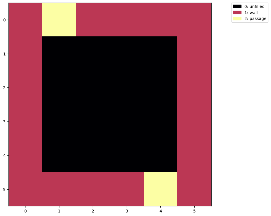
Very nice! We can see the starting and ending locations at (y=0, x=1) and (y=5, x=4).

Lay of the land

Instead of hard-coding the starting location and ending locations we can find them using numpy’s array.where method:

np.where(b == 2)

(array([0, 5]), array([1, 4]))

This gives us arrays with the y coordinates and the x coordinates of each location. For our program we need the y and x values for just one of these locations:

tuple(coord[0] for coord in np.where(b == 2))

(0, 1)

Next we collect the unfilled coordinates in the box:

np.where(b == 0)

(array([1, 1, 1, 1, 2, 2, 2, 2, 3, 3, 3, 3, 4, 4, 4, 4]),
 array([1, 2, 3, 4, 1, 2, 3, 4, 1, 2, 3, 4, 1, 2, 3, 4]))

Again we want the (y, x) coordinates not an array of y’s and an array of x’s so let’s swapaxes:

np.swapaxes(np.where(b == 0), 0, 1)

array([[1, 1],
       [1, 2],
       [1, 3],
       [1, 4],
       [2, 1],
       [2, 2],
       [2, 3],
       [2, 4],
       [3, 1],
       [3, 2],
       [3, 3],
       [3, 4],
       [4, 1],
       [4, 2],
       [4, 3],
       [4, 4]])

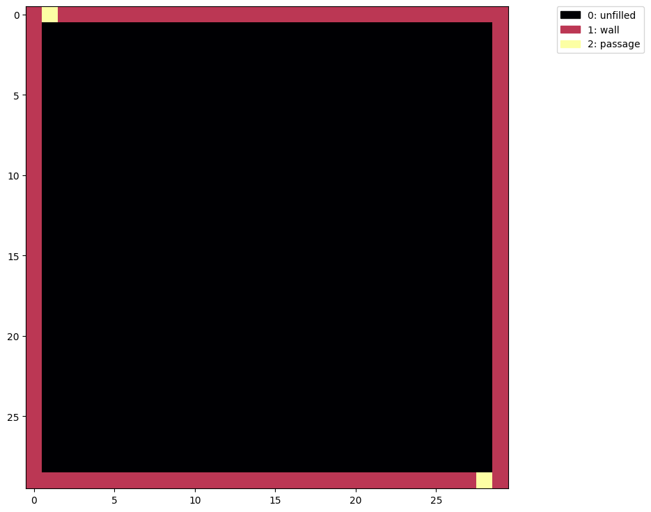
These are the coordinates that will become walls or passages in our maze, but first we’re going to need a bigger box, with many more coordinates to fill:

a = box(30, 30)
show(a)

The algorithm

Here’s our first flood fill maze generation algorithm “maze1”:

1. take all the unfilled coordinates and shuffle their order
2. save the starting coordinates (anything marked as a passage)
3. set all the existing passages to unfilled so the whole array is 0’s or 1’s.
4. for each of the unfilled coordinates
   • set it to a 1 (wall) and try flood filling the maze from the starting coordinates with 2’s (passage)
   • if any part of the maze remains a 0 (unfilled) then this wall has divided the maze making some part of it unreachable, so set the wall back to unfilled.
5. all remaining unfilled cells are part of the maze so set them to passages

def maze1(arr):
    unfilled = np.swapaxes(np.where(arr == 0), 0, 1)
    np.random.shuffle(unfilled)

    start = tuple(coord[0] for coord in np.where(arr == 2))
    arr = np.copy(arr)
    arr[arr == 2] = 0

    for lc in unfilled:
        lc = tuple(lc)
        arr[lc] = 1
        t = flood_fill(arr, start, 1)
        if np.any(t == 0):
            arr[lc] = 0

    arr[arr == 0] = 2
    return arr

show(maze1(a))

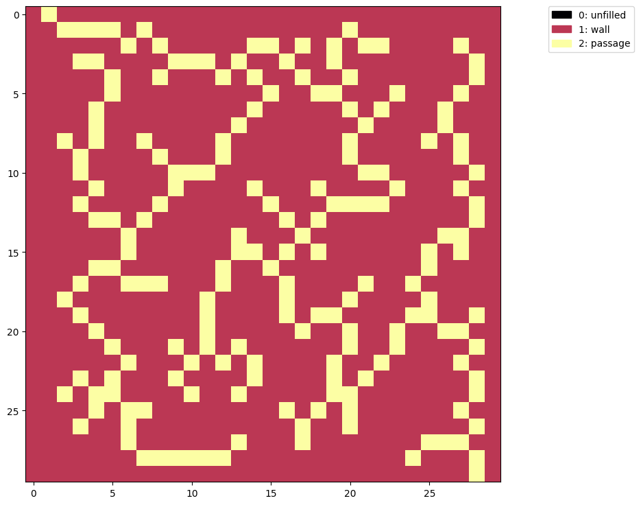
So that’s something. It is a maze, but I wasn’t expecting the maze to allow moving diagonally. Also it’s very sparse (mostly walls) and easy to solve.

The first problem is easy to fix. flood_fill has a connectivity parameter that sets the distance each cell can be from the next while allowing the fill to continue.

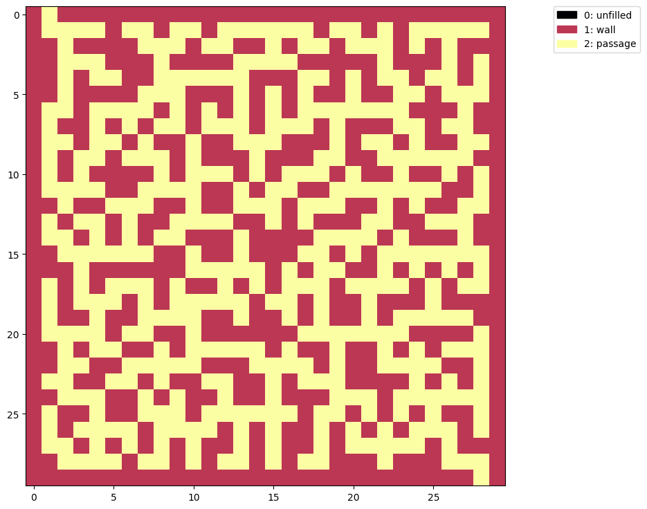
Here’s “maze2” like above but with connectivity=1:

def maze2(arr):
    unfilled = np.swapaxes(np.where(arr == 0), 0, 1)
    np.random.shuffle(unfilled)

    start = tuple(coord[0] for coord in np.where(arr == 2))
    arr = np.copy(arr)
    arr[arr == 2] = 0

    for lc in unfilled:
        lc = tuple(lc)
        arr[lc] = 1
        t = flood_fill(arr, start, 1, connectivity=1)  # no diagonals, please
        if np.any(t == 0):
            arr[lc] = 0

    arr[arr == 0] = 2
    return arr

show(maze2(a))

Better, but this maze is still very easy to solve.

Our algorithm sets every unfilled cell to a wall as long as that wall doesn’t cause the maze to be divided. So our walls end up very thick because any time a dead-end (a cell with three walls surrounding it) is selected it will be turned into a wall as well.

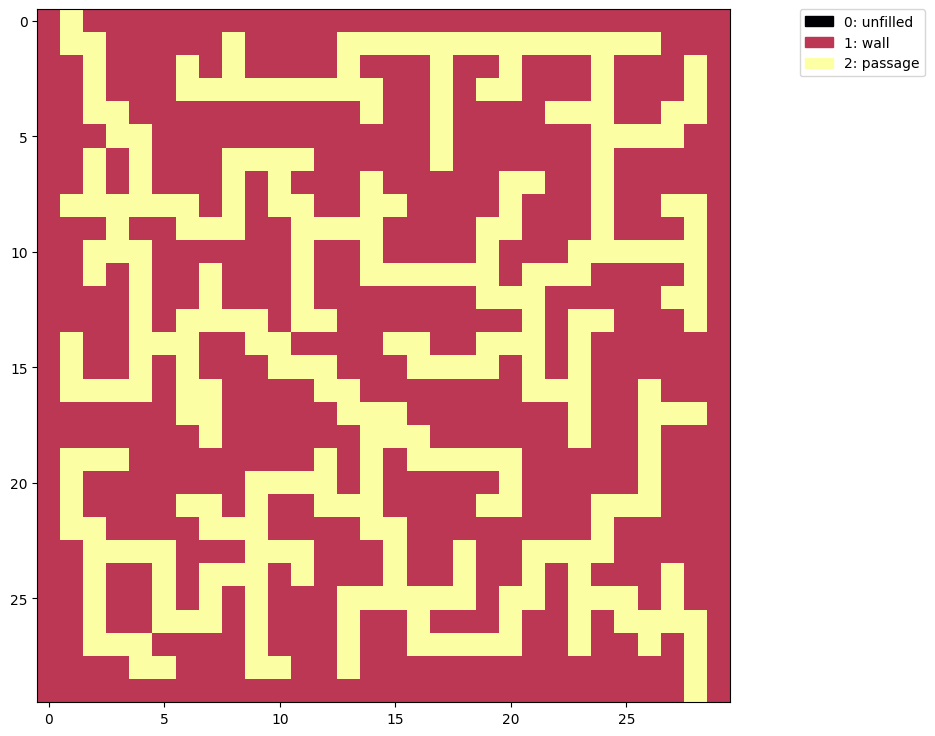
Let’s protect our dead-ends to generate more complex mazes with “maze3”:

# mask for cells above, below, left and right
neighbors = np.array([
    [0, 1, 0],
    [1, 0, 1],
    [0, 1, 0]], dtype=np.uint8)

def maze3(arr):
    unfilled = np.swapaxes(np.where(arr == 0), 0, 1)
    np.random.shuffle(unfilled)

    start = tuple(coord[0] for coord in np.where(arr == 2))
    arr = np.copy(arr)
    arr[arr == 2] = 0

    for lc in unfilled:
        lc = tuple(lc)

        y, x = lc
        # protect dead-ends from becoming walls
        if np.sum(neighbors * arr[y-1:y+2, x-1:x+2]) > 2:
            continue

        arr[lc] = 1
        t = flood_fill(arr, start, 1, connectivity=1)
        if np.any(t == 0):
            arr[lc] = 0

    arr[arr == 0] = 2
    return arr

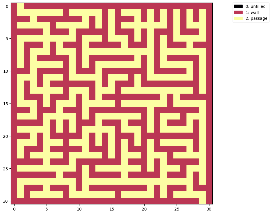
m = maze3(a)
show(m)

That’s more like it.

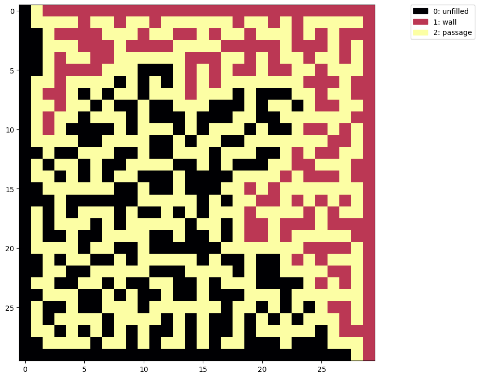
This maze has start and end positions on the edge so we can discover the path from start to end by flood-filling the walls one side and tracing the border between the two different colors:

# spoiler
t = flood_fill(m, (0, 0), 0)
show(t)

Spoiler

A “normal” maze

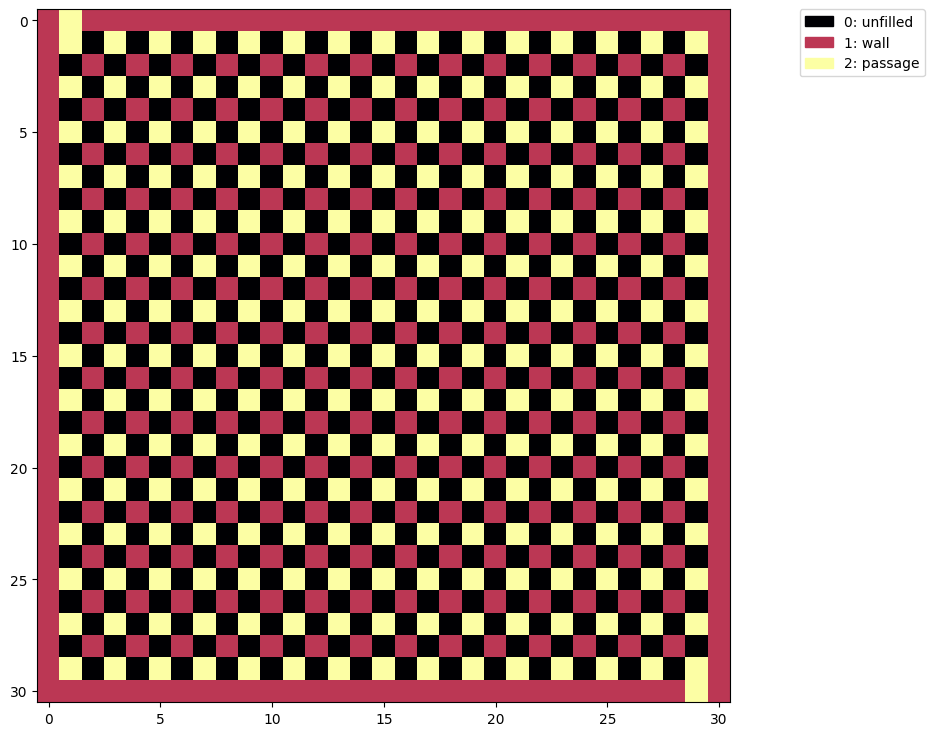
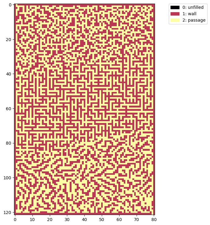
To generate mazes that look more like standard grid mazes we can start with a pattern of alternating passages and walls:

c = box(31, 31)
c[::2, ::2] = 1  # walls on even (y, x) values
c[1::2, 1::2] = 2  # passages on odd (y, x) values
show(c)

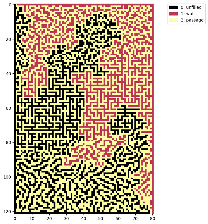
sm = maze3(c)
show(sm)

The same algorithm now produces a common grid maze, but we don’t have to stop there.

Big brain solution

Let’s take inspiration from nature and generate a maze from a brain coral image:

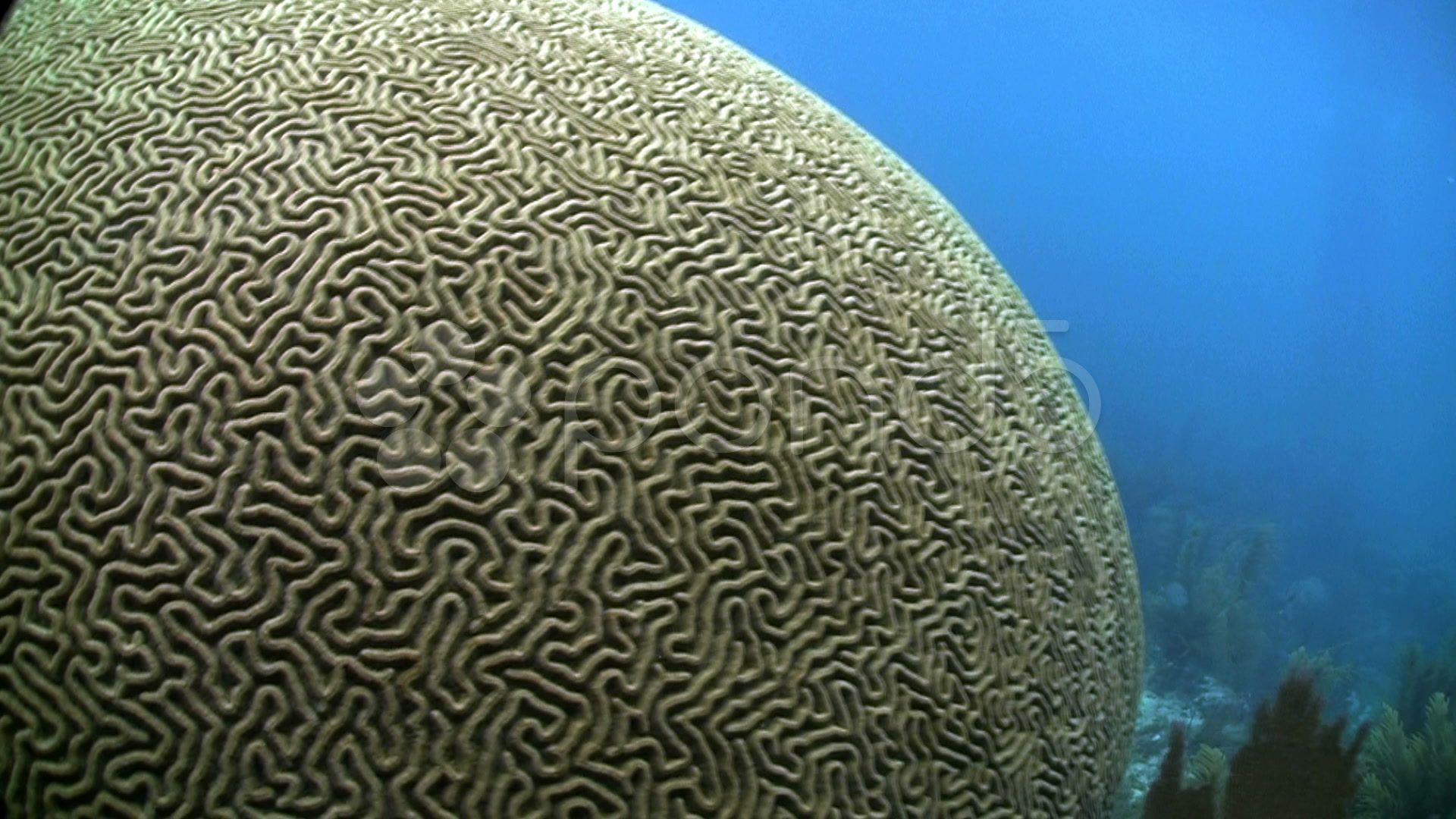
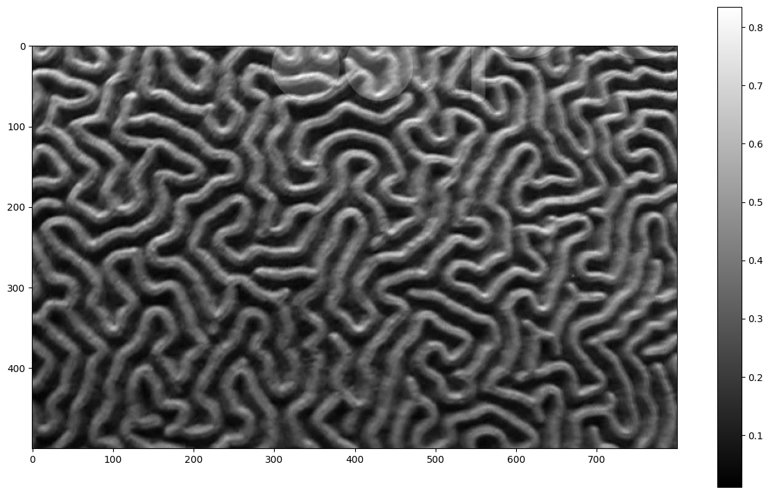
We load the image with imread then crop a small part and convert it to grayscale using rgb2gray:

brain = imread('brain-coral.jpg')
crop_brain = rgb2gray(brain[-500:,200:1000])
plt.figure(figsize=(15, 9))
im = plt.imshow(crop_brain, plt.cm.gray)
cb = plt.colorbar()

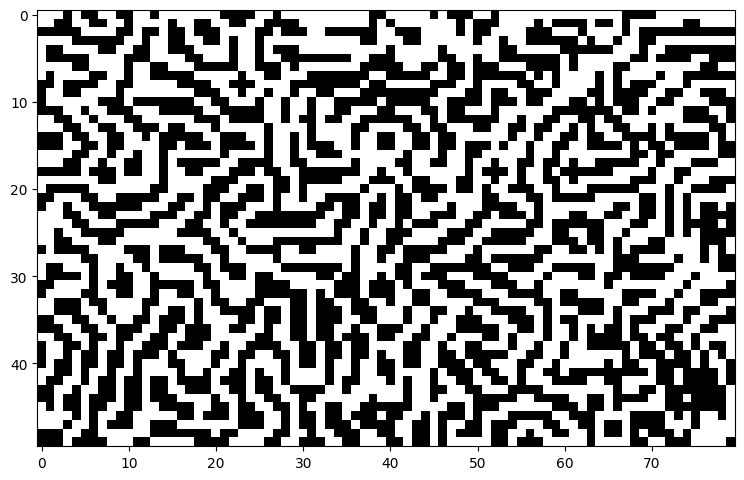
Next reduce the resolution with resize and use threshold_local to convert grayscale to 1’s and 0’s:

small_brain = resize(crop_brain, (50, 80))
binary_brain = small_brain > threshold_local(small_brain, 15, 'mean')
plt.figure(figsize=(9, 9))
im = plt.imshow(binary_brain, plt.cm.gray)

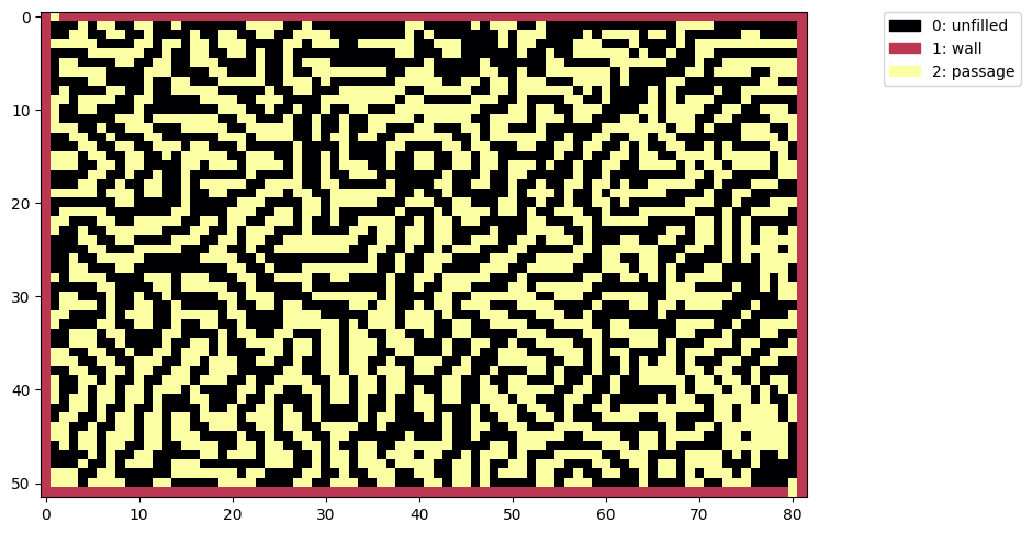
Then wrap the image with a box and turn the 0s into passages and the 1s into unfilled using modular arithmetic:

d = box(52, 82)
insert_brain = (binary_brain + 2) % 3
d[1:-1, 1:-1] = insert_brain
show(d)

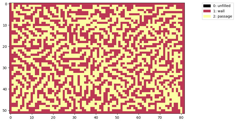
When we generate a maze with this pattern the walls can only be placed in the unfilled areas so our maze will follow the shape of the brain coral:

bm = maze2(d)  # maze2 is better: don't need lots of extra dead-ends
show(bm)

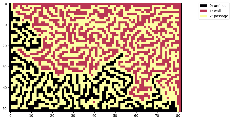
Here’s the solution:

# spoiler
t = flood_fill(bm, (0,0), 0)
show(t)

Spoiler

Why don’t we have both?

Drawing patterns for the algorithm to fill lets us create all sorts of mazes. If we save the grid and brain patterns with imsave we can use an image editor to combine them any way we like:

imsave('grid_pattern.png', palette[c])
imsave('brain_pattern.png', palette[d])

# use these to create combined_pattern.png with an image editing program

We can stitch patterns together and draw walls or passages through the image to shape the generated maze solution to any style and difficulty.

• combined_pattern.png

n = imread('combined_pattern.png')
# use red component to convert RGB to 0:unfilled, 1: wall, 2: passage
n = np.array((n[...,0] == 188) + (n[...,0] == 252) * 2, dtype=np.uint8)
show(n)

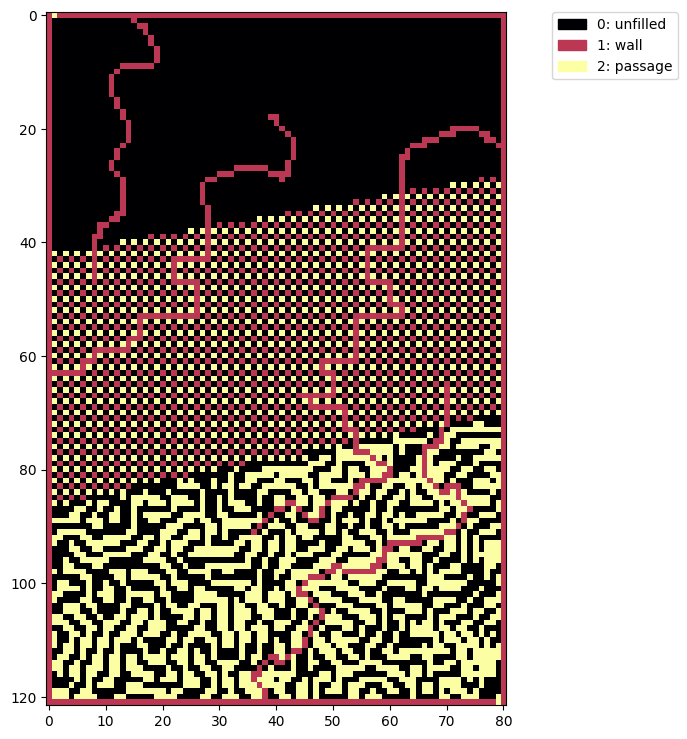
mn = maze3(n)
show(mn)

The solution follows our wandering path up and down through the different maze styles:

# spoiler
t = flood_fill(mn, (0,0), 0)
show(t)

Spoiler

This article showed how to generate mazes using jupyter notebooks, numpy, matplotlib, and the scikit-image flood_fill function.

The mazes started off very simple so we covered ways to increase the complexity and design custom patterns to shape the style and general path of the maze solution.

Thank you for reading!